5. Gapfilling Daily Weather Data

GWHAT provides an automated, robust, and efficient method to fill the gaps in daily weather data records. In addition, uncertainties of the estimated missing values can be automatically assessed with a cross-validation resampling technique. This document shows how to fill the gaps in daily weather records using the gapfilling weather data tool of GWHAT available under the tab Gapfill Weather shown in Fig. 5.1.

Fig. 5.1 Presentation of the gapfill weather data tool of GWHAT available under the tab Gapfill Weather.

5.1. Loading the weather data files

When starting GWHAT or when a new project is selected, the content of the Input folder is automatically scanned for valid weather data files that respect the format described in Section 3.2.1.

The restuls are displayed in a list located under Fill data for weather station section as as shown in Fig. 5.2. The list of weather datasets can be refreshed at any times by clicking on the icon. This needs to be done if new datafiles are added or deleted manually from the Input folder, outside of GWHAT. Datasets can be removed from the list by selecting them and clicking on the icon. Doing so also removes the corresponding data file from the Input folder.

A summary of the number of days with missing data for each dataset is also produced and displayed under Missing Data Overview tab of the display area.

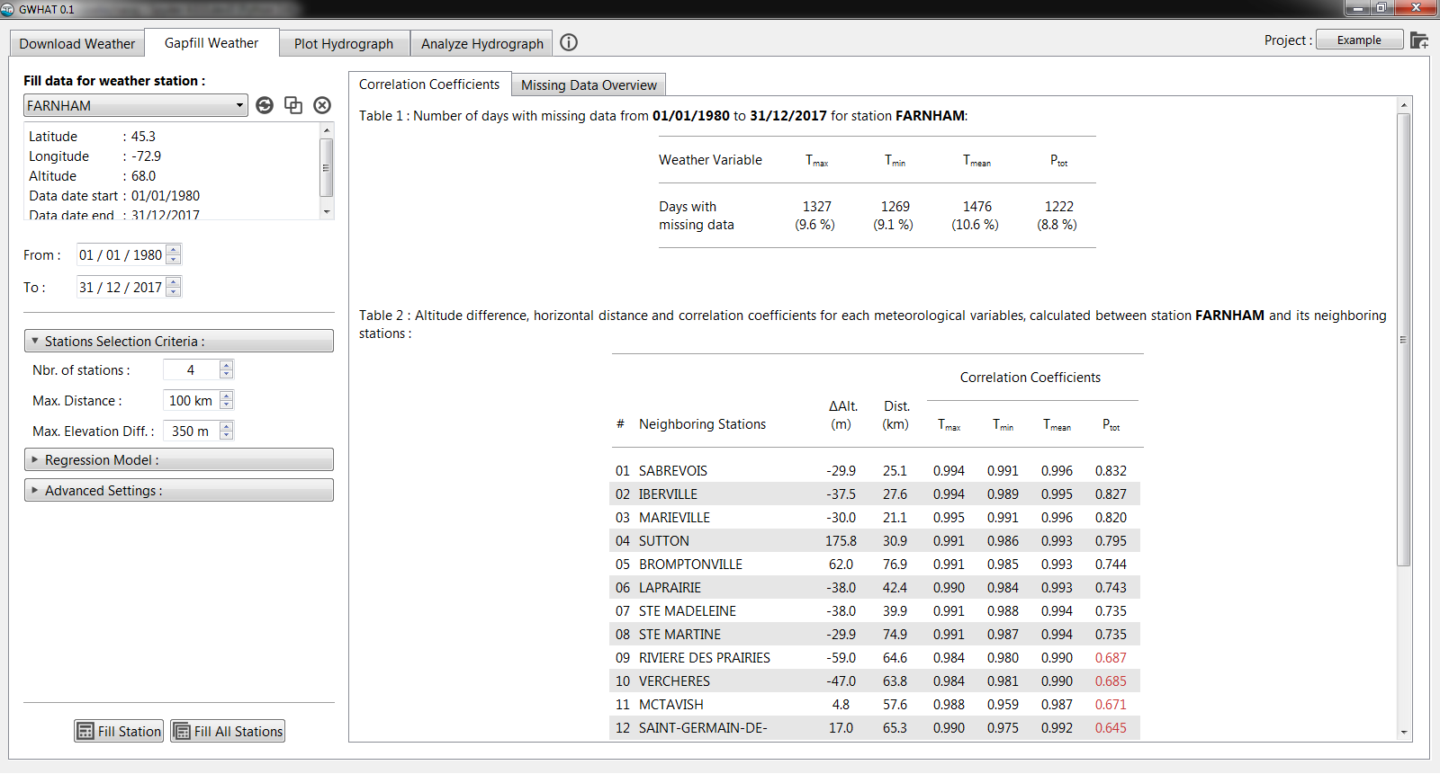
Fig. 5.2 Presentation of the gapfill weather data tool of GWHAT available under the tab Gapfill Weather.

5.2. Merging two weather data files

Sometimes, more than one daily weather dataset is available at a same location. Often, this happens when a new climate station is installed in a location where a station was operating in the past, but was later removed (due to governmental budget cuts for example). This results in two datasets for which the data are mutually exclusive in time. In that case, it is beneficial to merge these two mutually exclusive datasets into a single dataset that spans over a longer period of time. This can be done mannually by manipulating the files located in the Input folder or by using the tool available in GWHAT by clicking on the icon (see Fig. 5.3).

Fig. 5.3 Presentation of the tool to merge two daily weather records together.

Note

Datasets that are mutually exclusive in time can results in problems when filling the gaps in daily weather records. So it is always a good practice to reduce the occurence of the situation described above in the input weather datafiles before trying to fill the gaps in the data.

5.3. Filling the gaps in the data

The first step is to select the dataset for which missing values need to be filled. This is done from the drop-down list located under the Fill data for station section shown in Fig. 5.2. Under this list are displayed information about the currently selected weather station.

It is also possible to define the period for which the data of the selected station will be filled by editing the date fields located next to the From and To labels. By default, dates are set as the first and the last date for which data are available for any of the stations of the list.

The method used to estimate the missing data for the selected weather station consists in the generation of a multiple linear regression (MLR) model, using synchronous data from the neighboring stations. The neighboring stations used to generate the MLR model are selected based on the correlation coefficients computed between their data and those of the selected weather station. The values of these coefficients are automatically calculated when a new weather station is selected from the dropdown list and the results are displayed in the table located under the Correlation Coefficients tab. Among the selected neighboring stations, the ones with the highest correlation coefficients have more weight in the model than those with weak correlation coefficients. As a guidance for the user, correlation coefficients that fall below a value of 0.7 are shown in red in the table. There are several settings that can be used to control the selection of the neighboring stations, the generation of the MLR model, and the outputs of the gapfilling procedure. An overview of these settings is presented below in Section 5.5.

Once the parameters have been set to the desired values, the automated procedure to fill the gaps in the dataset of the selected climate station can be started by clicking the button Fill. It is also possible to fill the gaps of all the datasets of the Fill data for weather station dropdown list in batch by clicking on the button Fill All Stations. The parameters used in the gapfilling procedure will then be the same for all the stations.

5.4. Output files

Once the process to fill the gaps is completed for a station, the resulting gapless daily weather dataset is automatically saved in a csv file with a .out extension in the Output folder. Detailed information about the format of the .out files are provided in Section 3.2.1. The .out file is named after the weather station name, climate ID, and first and last year of the dataset. For example, the resulting output file for the station FARNHAM in Fig. 5.2 would be FARNHAM (7022320)_1980-2017.out.

Detailed information about the estimated values that were used to fill the gaps in the data series (e.g., parameter values used in the method, uncertainty of the estimated values, simultaneous data at neighboring stations used for the estimations) are also saved in an accompanying file with a .log extension. A histogram showing the yearly and monthly weather normals, calculated from the gapless data series is also produced and saved in a pdf format. An example is presented in Fig. 5.4.

Additional outputs are produced when the option Full Error Analysis is checked in the Advanced Settings (see Section 5.5.3). These outputs are described in more details in Section 5.6.

Fig. 5.4 Example of a histogram generated by GWHAT showing the yearly and monthly weather normals for the climate station MARIEVILLE.

5.5. Setting the parameters

This section describe the various parameters that can be set to control the selection of the neighboring stations, the generation of the MLR model, and the outputs of the gapfilling procedure.

5.5.1. Stations Selection Criteria

A MLR model is generated for each day for which a data is missing in the dataset of the selected station. This is done because the number of neighboring stations with available data can vary in time. Therefore, for a given date with missing data in the dataset of the selected station, the neighboring stations are selected in decreasing order of their correlation coefficients. Neighboring stations that also have a missing data at this particular date are excluded from the selection process.

The maximum number of station that are selected for the generation of the MLR model can be specified with the parameter Nbr. of stations, located under the Stations Selection Criteria section shown in Fig. 5.5. The number of neighboring station that is selected by default is 4. If for a given date, all the neighboring stations have missing data synchronously with the selected station, a nan value is kept in the dataset at this particular date.

Moreover, the correlation between the data of two stations generally decreases as the distance and the altitude difference between them increase. Therefore, the parameters Max. Distance and Max. Elevation Diff. allow to specify thresholds for the distance and altitude difference. Neighboring stations exceeding either one of these thresholds will not be used to fill the gaps in the dataset of the selected station. The default values for the distance and altitude difference are set to 100 km and 350 m, respectively, based on values found in the literature (Simolo et al., 2010; Tronci et al., 1986; Xia et al., 1999). The horizontal distances and elevation differences calculated between the selected station and its neighbors are shown in the table to the right, alongside the correlation coefficients. The values that exceed their corresponding threshold are shown in red.

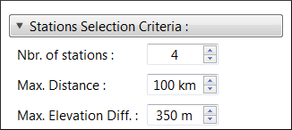
Fig. 5.5 Parameters that can be set to control the selection of the neighboring stations in the gapfilling procedure.

5.5.2. Regression Model

It is possible to select whether the MLR model is generated using a Ordinary Least Squares (OLS) or a Least Absolute Deviations (LAD) criteria from the Regression Model section shown in Fig. 5.6. A regression based on a LAD is more robust to outliers than a regression based on a OLS, but is more expensive in computation time.

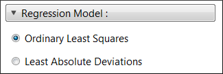
Fig. 5.6 Parameters to control the criteria used to generate the MLR model.

5.5.3. Advanced Settings

It is possible to automatically estimate and add the daily Potential Evapotranspiration (PET) to the output data file (.out) produced at the end of the gapfilling procedure of the selected station. This option is enabled by checking the Add PET to data file option in the section Advanced Settings shown in Fig. 5.7. The daily PET is estimated with a method adapted from Thornthwaite (1948), using the daily mean air temperature time series of the selected station. Alternatively, it is possible to add manually the PET retrospectively to an existing .out file by clicking on the icon.

The Full Error Analysis option can be checked to perform a cross-validation resampling analysis during the gapfilling procedure. The results from this analysis can be used afterward to estimate the accuracy of the method. This option is discussed in more details in Section 5.6.

Finally, the format (pdf or svg) and the language (English or French) of the figures that are automatically produced by GWHAT after a dataset has been sucessfully gapfilled (see Fig. 5.4 and Fig. 5.8) can be selected from the Figure output format and Figure labels language menus.

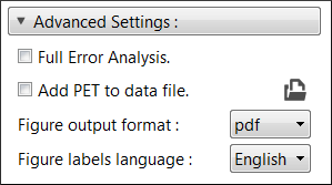
Fig. 5.7 Advanced parameters of the gapfilling procedure.

5.6. Uncertainty Assessment

By default, each time a new MLR model is generated to estimate a missing value in the dataset of the selected station, the model is also used to predict the values in the dataset that are not missing. The accuracy of the MLR model is then approximated by computing a Root-Mean-Square Error (RMSE) between the values estimated with the model and the respective non-missing observations in the dataset of the selected station. The RMSE thus calculated is saved, along with the estimated value, in the .log file.

When the Full Error Analysis option in the Advanced Settings section is checked, GWHAT will also perform a cross-validation resampling procedure to estimate the accuracy of the model, in addition to fill the gaps in the dataset. More specifically, the procedure consists in estimating alternately a weather data value for each day of the selected station’s dataset, even for days for which data are not missing.

When a value for every day of the dataset has thus been estimated, the estimated values are saved in the Output folder as a csv file with a .err, along with the .log and .out files as described in Section 5.3. The accuracy of the method can then be estimated by computing the RMSE between the estimated weather data and the respective non-missing observations in the original dataset of the selected station.

In addition various graphs are automatically generated by GWHAT to the performance of the method and saved in a pdf format. These graphs consist of scaterplots comparing the estimated and measured daily weather data and a plot comparing the probability density function of the original and the estimated daily precipitation series. Example of these graphs are presented in Fig. 5.8.

Fig. 5.8 Graphs that are automatically generated by GWHAT allowing to assess the performance of the method to fill the gaps in daily weather data records accurately.

Note

Checking the Full Error Analysis option will increase the computation time of the gap filling procedure, especially if the least absolute deviation regression model is selected, but can provide interesting insights on the performance of the procedure for the specific datasets used for a project.