6. Plotting the Hydrographs

This document shows how to produce publication quality figures of well hydrographs in GWHAT using the tools available under the tab Plot Hydrograph shown in Fig. 6.1. For detailed information on how to import the weather and water level data in GWHAT, please consult Section 3.

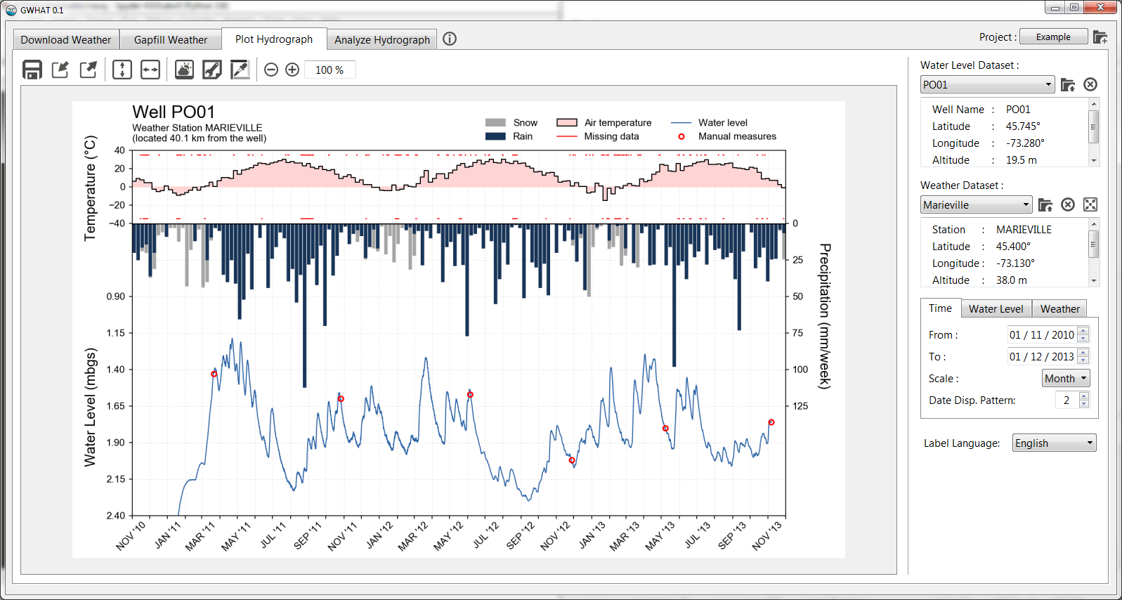
Fig. 6.1 Presentation of the tool to plot hydrographs in GWHAT under the Plot Hydrograph tab.

The tab Plot Hydrograph consists mainly of an editor to produce a graph showing the groundwater level time series in relation to weather conditions. As shown in Fig. 6.2, the editor consists of a toolbar, the panel Input data (documented in Section 3), the panel Axes settings, and a canvas where the hydrograph figure is shown.

A figure of the hydrograph is produced as soon as a water level dataset have been selected in the Input data panel. It is possible to zoom the figure canvas in or out by pressing the or icon or by rotating the mouse wheel while holdind the Ctrl key.

Various parameters are available to customize the layout of the hydrograph:

• Several options are available to customize the size and visibility of the components of the hydrograph in the Page and Figure Setup window, which is accessible by clicking on the icon. This is covered in more details in Section 6.2.
• The color of most of the elements that are plotted in the hydrograph can be configured in the Colors Palette Setup window, which is accessible by clicking on the icon. This is covered in more details in Section 6.4.
• The axis of the graph can be configured in the Axes settings panel. This is covered in more details in Section 6.3. In addition, the and icons can be clicked at any time to, respectively, fit the time and water level axis automatically to the data.
• The icon is used to access the Weather Averages window where are displayed the yearly and monthly normals of the weather dataset. This is covered in more details in Section 7.

The layout for the currently selected water level dataset can be saved by clicking on the icon. The previously saved layout can be loaded back for the currently selected water level dataset by clicking on the icon. Finally, the hydrograph can be saved in a pdf, svg or png format by clicking on the icon.

Fig. 6.2 Presentation of the editor to produce publication quality figures of well hydrographs that is available in the tab Plot Hydrograph of GWHAT.

6.1. Components of the Hydrograph

Fig. 6.3 presents the various elements of the hydrograph. Each of these are discussed in more details below.

Fig. 6.3 Identification of the components of the hydrograph.

6.1.1. Observed water levels

The observed water levels are plotted on the bottom part of the hydrograph. By default, groundwater levels are represented by a continuous line that connects to all available data.

It is possible to ensure that the continuous line is not drawn over periods where data is missing by marking the missing period in the water level time series with at least one nan value before importing the water level dataset in GWHAT. For example, in Fig. 6.4, water levels were missing for the whole of 2012. A nan was thus added in the time series at one time during this period to avoid a line to be plotted between the 31/12/2011 and the 01/01/2013.

Fig. 6.4 Example of an hydrogaph with an extended period of time for which data is missing.

As shown in Fig. 6.5, it is also possible to show the trend of the water level by setting the option Water Level Trend to On in the Page and Figure Setup window (see Section 6.2). The actual observed data are then plotted under the trend line as a scatter plot. The trend line is computed using a moving average window of 30 days.

Fig. 6.5 Example of a hydrograph where the trend of the water level is shown as a continuous blue line along with the real observations plotted as a series of light gray dots.

6.1.2. Weather data

Mean air temperature is plotted in the top part of the graph. The area between 0ºC and the observed temperature is colored by default to highlight the periods when air temperature is below the freezing point of water. Mean air temperature can be plotted on a daily, weekly, or monthly basis. This can be changed from the Axes settings panel as discussed in Section 6.3.

Cumulative precipitation, as rain and snow, is plotted in the bottom part of the hydrograph along with the water level data. For a given day, precipitation is assumed to fall as snow if the mean air temperature for that day is below 0ºC and as rain otherwise. As for air temperature, cumulative precipitation can be plotted on a daily, weekly, or monthly basis.

As shown in Fig. 6.5, it is possible to plot the water level data alone, without the mean air temperature and cumulative precipitation, by setting the Weather Data component to Off in the Page and Figure Setup window.

6.1.3. Missing weather data

The Missing data component is used to mark where daily air temperature and precipitation were estimated due to missing data in the dataset. This information is read when importing a dataset in GWHAT (see Section 3.1) from the .log file that is produced automatically when gap filling daily weather records with the tool presented in Section 5.

Note

If no .log exists when importing a daily weather datafile in GWHAT, Missing data markers won’t be plotted on the hydrograph, even if data are missing in the daily weather dataset.

6.1.4. Water level manual measurements

Water levels measured manually during field visits can also be plotted on the hydrograph. This provides a quick and easy way to visually validate the automated measurements acquired with a water-level data logger.

To do so, the manual measurements must be saved in a csv or xls/xlsx file named water_level_measurements in the Water Levels folder (see Section 2.3). An example is shown in Fig. 6.6 below. The first column corresponds to the name of the observation wells (see Section 3.1), the second column is the dates entered in Excel numeric date format, and the last column corresponds to the manual measurements, in metres below the ground surface.

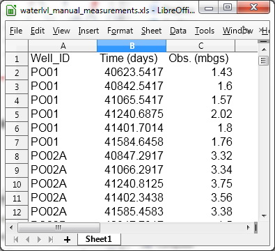
Fig. 6.6 Example of a water_level_measurements file.

Note

A water_level_measurements file is created in a csv format by default by GWHAT the first time a project is created. If desired, this file can be converted to a xsl or xslx format. Note that if more than one file named water_level_measurements exists in the folder Water Levels, but with different extension, GWHAT will always read the data from the csv file by default.

6.1.5. Water level envelope predicted with GLUE

Water levels predicted by optimizing a quasi-two-dimensional hydrologic model with the GLUE (Generalized Likelihood Uncertainty Estimation) methodology at the 05/95 uncertainty level can be plotted on the hydrograph once groundwater recharge have been evaluated with the tool presented in Section 10.

As for many other elements of the hydrograph, the plotting of the GLUE predicted water level envelope can be turned on or off in the Page and Figure Setup window.

6.2. Page and figure settings

Several options are available to customize the size and visibility of the various components of the hydrograph in the Page and Figure Setup window, which is accessible by clicking on the icon (see Fig. 6.2). The Page and Figure Setup window is shown in Fig. 6.7, along with an annoted figure where are presented the various components of the hydrograph layout that can be configured from this dialog.

Fig. 6.7 Presentation of the components of the hydrograph for which the size or the visibility can be configured in the Page and Figure Setup window.

6.3. Axis settings

The scale and range of the axes for time, water level, and weather data can be configured from the Axes settings panel, located on the right side of the hydrograph editor. The options that are available for each axis are presented in Fig. 6.8. The hydrograph is updated automatically when a value is changed in the Axes settings panel.

6.3.1. Time axis

The range of the time axis can be changed by setting the From and To dates. The Scale of the time axis can be set to monthly or yearly. The Date Disp. Pattern setting allows to define the interval with which the tick labels of the time axis are plotted. Four different cases with different values of the Scale and The Date Disp. Pattern settings are presented in Fig. 6.8.

6.3.2. Water levels axis

The Minimum setting of corresponds to the value at the bottom of the water level axis. The Grid Divisions value corresponds to the number of intervals in which the water level axis is divided as shown on Fig. 6.8. The Datum of reference of the water level axis can be set to either Ground Surface or Sea Level.

The value at the top of the water level axis is calculated from the values specified in Minimum, Scale, and Grid Divisions. The equation that is used in the calculation, which depends on the Datum that is selected, is presented at the bottom of Fig. 6.8.

6.3.3. Weather axis

Only the scale of the axis for the precipitation is configurable through the Precip. Scale setting. The minimum value for precipitation is always set to 0 and the range of the axis depends on the value specified for the setting Precip. Scale and Grid Divisions in the water level axis settings.

As discussed in Section 6.1.2, the Resampling setting is used to set the time scale on which mean air temperature and cumulative precipitation are plotted on the graph.

6.4. Color Settings

The color of several components of the hydrograph can be changed from the Colors Palette Setup window, which is accessible by clicking on the icon (see Fig. 6.2). The Colors Palette Setup window and the components of the hydrograph for which the color can be changed are both shown in Fig. 6.9. A new color can be selected for a given component of the hydrograph by clicking on its corresponding colored square in the Colors Palette Setup window and by clicking on the OK or Apply button.

Fig. 6.9 Presentation of the Colors Palette Setup and identification on the hydrograph of the components for which the color can be changed.